

In the Part I article, we provided the background of recursive proofs and how they are important in Stwo to scale to unbounded computation. We worked with StarkWare to build a recursion system for Stwo, which consists of two components: Plonk and Poseidon.
We already presented the details of the Plonk component and how it can be used to represent different kinds of arithmetic relationships and therefore can be used to verify all kinds of computation. In this article, we will focus on the other component, Poseidon, which indeed has a much trickier and more intricate design.
The full recursive proof generation for Stwo has completed, and one can find the related source code in GitHub:
Proof systems: https://github.com/Bitcoin-Wildlife-Sanctuary/stwo-circle-poseidon-plonk
Recursion circuits: https://github.com/Bitcoin-Wildlife-Sanctuary/recursive-stwo
Bitcoin verifier: https://github.com/Bitcoin-Wildlife-Sanctuary/recursive-stwo-bitcoin
We now dive into the detail of the Poseidon component of the proof system.
The role of hash functions in STARK
We just mentioned that the Plonk component, which was already discussed in the Part I article, can represent all kinds of computation, which, of course, also includes Poseidon hash functions. One may be curious about why we need a dedicated Poseidon component in the proof system, as one can just use Plonk to take care of the same computation.
The reason is about the cost of verifying Poseidon in Plonk. Throughout the entire STARK proof verification as part of the recursion, there are several places that involve hash functions, as shown in the figure below.

STARK uses Fiat-Shamir transform, which is used to generate the randomness in the zero-knowledge proof. This transform uses the output of the hash functions for such randomness. The specific procedure of the Fiat-Shamir transform has to do with the “size” of the proof system and the circuit. When the proof system that is being recursively verified has a lot of columns, the Fiat-Shamir transform may end up invoking hash functions a lot.
Then, STARK also uses proof-of-work (also known as grinding) as an optimization for verifiers. This would also require the verifier to compute the hash function, but it is usually only once.
What follows Fiat-Shamir transform and proof-of-work is all about Merkle trees—during STARK proof generation, some data is committed into Merkle trees, and the verifier opens the Merkle trees on random locations to check if the data matches up. This would constitute the majority overhead involving hash functions because STARK proof verification needs to open a number of Merkle trees, and since the check needs to be conducted on many random locations, the process is repeated a few times.
Experiments show us that, when doing recursive proof verification, the overhead involving hash functions can easily become the dominating overhead. This needs to be taken care of because we want to, eventually, verify the Stwo proof on Bitcoin or Ethereum, and this requires us to be able to recurse a larger proof into a small proof. If the recursion circuit is too complicated, one may run into the problem that recursion ends up increasing the verification overhead because the recursion circuit is larger than most applications that we care about.
Now that we have discussed why Poseidon requires more dedicated efforts instead of using Plonk to compute Poseidon hash functions directly, we want to talk about its overhead and how making dedicated columns can help verify Poseidon hash functions faster.
Poseidon hash function
The hash function that we use is Poseidon2. Today, this is a well battle-tested hash function that becomes almost the crown prince, especially because many other ZK-friendly hash functions, including Griffin, Arion, Anemoi, Rescue, have been shown to be weaker than originally expected and need larger parameters (see [1], [2], [3]).
We instantiate the Poseidon2 hash function over the Mersenne-31 field. Each input or output consists of two parts following the sponge construction: one called rate that is expected to be public, and one called capacity that is expected to remain private.
To achieve 128-bit security, each rate and capacity needs to be at least (around) 256 bits, so we set the rate and capacity to each consist of 8 elements of M31. That is to say, the input or output to the hash function would have 16 elements of M31, as shown below.

Poseidon2 will perform a sequence of transformations on the input to generate the output. At a high level, it starts with some linear transformation that preprocesses the input, and then it continues with 4 full rounds, 14 partial rounds, and then 4 full rounds.
Note that the full rounds are the first 4 and the last 4 rounds of such transformations. This is why it also receives the name “external” rounds, as they encapsulate the 14 partial rounds in the middle, which is also called “internal” rounds for this reason.
Full rounds differ from partial rounds, in that full rounds perform more heavy computation, while the partial rounds are more lightweight—nevertheless, there are more partial rounds. Since we will need to go into the detail of our Poseidon component, we now should discuss how the full rounds and partial rounds work.
Full round. In Poseidon2, a full round performs three steps.
Add the current state (rate and capacity, in total 16 elements) with round constants, which are round-specific, fixed but random M31 elements.
Apply S-box to each element of the state. In our case, the S-box maps x to x^5.
Perform a linear transform with a 16x16 MDS matrix.
The first step and the last step are linear transformations (additions and multiplications by known and fixed constants), and representing them in ZK circuits is straightforward. The second step involves a degree-5 arithmetic transformation.
Previously, if we use Plonk to represent such relations, we run into the issue that each row in the Plonk component can either do one addition or one multiplication, and therefore, the full round would generate a number of rows.
The first step, adding round constants, would basically generate 16 rows, while each row adds one element in the state by a corresponding constant.
The second step, applying the S-box, would contribute 48 rows, while every three rows takes care of mapping one element from x to x^5.
The last step, performing the MDS matrix, might be most expensive, as it would contribute 120 rows.
This adds up to 184 rows per full round. We will show, later in this article, how to do 2 full rounds in one row in the Poseidon component.

Partial round. The computation in full rounds is called “full” in that each and every element in the state (in total 16 elements) gets the S-box. Since S-box consumes more compute resources than the rest of the operations because it involves multiplication while the rest can be mostly implemented through additions, researchers have decided to reduce the use of S-box while preserving the security, at the cost of having more rounds (more frequent “diffusion”).
So, in Poseidon2, other than the 4 full rounds at the beginning and 4 full rounds at the end, there are also 14 partial rounds lying between them (and therefore called the internal rounds). It also has three steps, but the computation at each step is much more lightweight:
Add the *first element* of the current state with a round constant, while the remaining 15 elements stay unchanged.
Apply the S-box to only the *first element* while keeping the rest of the elements unchanged.
Perform a linear transformation that is a lightweight matrix.
Implementing a partial round in Plonk is possible, and the cost would be smaller than a full round, but still a lot.
The first step generates only one row.
The second step generates only three rows.
The last step involves 47 rows.
This adds up to 51 rows per partial round, and there are 14 such rounds. However, we can do much better than this. We will later show how to do 14 partial rounds in a single row in Stwo with the Poseidon component.

Idea for optimization
Before we present our construction of the Poseidon module, we first want to discuss how to optimize from the baseline (using Poseidon) and why such an optimization is possible.
Remember from the Part I article that the overhead for the prover is dominated by the number of columns times the number of rows (in other words, the number of cells in the proof system).
When we use the Plonk proof system to represent the computation, remember that each row can perform one addition or one multiplication, and each row has 10 + 12 + 8 = 30 columns. Based on our computation above, the entire Poseidon evaluation requires 2186 rows, and correspondingly 65580 cells.
This is in contrast to the construction that we will show later, which uses 6 rows in the Poseidon component, where the Poseidon component has 96 columns. This only uses 576 cells, reaching an improvement on prover time by at least 114x.
There are many reasons that contribute to the slowdown of the baseline approach, but we can summarize them into two aspects:
The Plonk proof system has too many columns that are underutilized when running a Poseidon function.
The Plonk proof system cannot represent linear operations in the Poseidon function efficiently.
Underutilization. Remember that the Plonk proof system that we discuss uses QM31 as elements. However, the Poseidon2 hash function that we use is defined over M31. This already means that out of the 12 “trace” columns, 9 of them are dummy and would all be zero.
Then, remember that the rest of the Plonk proof system is taking care of passing variables from one row to another. A lot of columns are actually used for this purpose. For example, among the 10 preprocessed columns, three columns “a_wire”, “b_wire”, “c_wire” are used to give an identifier for the A, B, C variables, and three columns “mult_a”, “mult_b”, “mult_c” are used for the logUp arguments. For each row, we also have 8 interaction columns for logUp.
This means that, when we perform additions over 16 elements, we need 16 rows, and each row would require independent and dedicated logUp columns. But, in fact, these 16 elements are processed often in a batch, and, being intermediate variables of the hash function computation, they would not be used in other places in the proof system, but just immediately consumed by subsequent rounds (the 4+14+4 rounds in the Poseidon) function. The power of the logUp argument to pass variables to any other rows in the proof system, for an arbitrary number of times, is an overkill.
One can think of the Plonk proof system as a very generic purpose CPU that has a random access memory—data can be read or written for arbitrary number of times, at any place of the program—and also a high CPU word size that processes 4 elements at the same time, but we often only use one element in evaluating the Poseidon hash function. This CPU is unaware of the batch operations that we are performing, and it gets and puts each element within the batch treating them as unrelated.
We address such underutilization, informally, by designing the Poseidon proof system as a dedicated CPU that performs operations in batch, including batch access to the memory, with also less frequent access to the memory by doing more computation steps between each access. It processes 16 elements each row. Before it uses the logUp argument, it either applies 2 full rounds in this row, or applies 14 partial rounds in this row, while previously even a single round may have 51 to 184 rows.
We will present the details very soon, but one can see that eliminating the redundancy and underutilization of the Plonk proof system can materially reduce the prover cost.
Inefficiency. The other reason for the slowdown is that it doesn’t represent the linear relations in the most efficient way. For example, consider a full round. If we use the Plonk proof system to implement the full round, all the three steps of the full round—adding round constants, applying S-box, and performing linear transform—all contribute to rows, and we know that the linear transform contributes the most. These rows lead to cells, which lead to prover inefficiency. From our previous computation, a full round leads to 5580 cells.
However, if we only focus on the computation related to the full round, in the purest form, this seems doable with only 48 cells, 16 cells for the round constants, 16 cells for the input, and 16 cells for the output. Note that round constants are preprocessed columns that the prover doesn’t have to commit every time.

The equation between these columns are, of course, more complicated—it is degree-5, it involves a lot of variables, but it is indeed very easy to verify.
Additions are very efficient to compute.
All the weights (w_{i,j} in the figure) are all very small values, and there are algorithms to evaluate this (the MDS matrix) very efficiently.
By using these equations to handle the 16 elements altogether, the number of the cells involved in the computation is significantly lower—in the example above, you can see that adding round constants does not introduce additional columns (other than the round constants preprocessed columns that the prover doesn’t need to compute), and the linear transform via the MDS matrix contributes to no columns as well.
The same applies to partial rounds. Applying the same rule of thumbs, we know that for each partial round, adding the round constant (which only involves the *first element*) only requires one preprocessed column, but no other columns, and the linear transform would involve no column. In this way, processing 14 rounds needs just about 14 + 16 + 16 = 46 columns.
Since 46 is smaller than 48, we can actually let the full rounds and partial rounds share the columns. Some rows will be for “full rounds”, so these columns are used for the full-round computation, while the other rows will be for “partial rounds”, where the same columns are instead used for partial-round computation.
Our construction
We here present the high-level construction of the Poseidon component, but we skip the detail about the logUp argument, which we already discussed in the Part I article. We will present a simplified version, and readers who want to learn about the full version can look at our implementation here in GitHub.
Each invocation of the Poseidon hash function would create 6 rows in the Poseidon component. There are two control columns, “First round?” and “Full round?”, that are changing in these 6 rows, and they directly impact how the 48 columns of input, intermediate, outputs are used.

The first row performs a linear transform (the MDS matrix) on the input, skipping the S-Box or round constants. This is a standard and necessary preprocessing step in Poseidon2. In recent years, doing so is known to be important for security.
After the first row, we have the second row and the third row for the first 4 full rounds, where each row takes care of two full rounds altogether. Within each row,
The first full round applies to the 16 input columns and writes its output to the 16 intermediate columns.
The second full round applies to the 16 intermediate columns and writes its output to the 16 output columns.
The logUp argument, which we skip here, is in charge of connecting the output of the first row (the input after the linear transformation) to the input of the second row, and so on and so forth.
The fourth row, which has both “First Row?” and “Full round?” set to zero, will complete all 14 partial rounds. We store the result after the first 4 full rounds in input, and we store the result after the 14 partial rounds in output. As for the intermediate columns, we use 14 out of 16 of them to store the first element after the S-box in each round, due to some technical necessity to do so.
Then we continue with another two rows, each taking care of 2 full rounds. So, we have completed all the 4 + 14 + 4 rounds of the Poseidon hash function.
There are some other columns and logic in the Poseidon component in our implementation that we are not presenting here: they take care of the inputs and outputs between the rows and with the Plonk component (through the logUp arguments discussed in the Part1 article). We also let the Poseidon component take care of swapping the first half and second half of the inputs given a bit, which is mostly used for Merkle tree path verification. The details of such extensions can be found in the code, but each Poseidon evaluation still only contributes to 6 rows.
Writing the recursion circuits
The full proof system for recursion proof verification in Stwo is the combination of the Plonk component and the Poseidon component. We program primarily in the Plonk component, and only when we use the Poseidon hash function, it programs in both components.
We write the recursion circuits in Rust, using a DSL similar to the one that we used to write Bitcoin scripts (which we discussed in a previous article). This DSL allows us to convert existing Rust code in the StarkWare’s Stwo library into the DSL code for circuits.
For example, in the Poseidon component, we need to perform the linear transformation in a full round, the corresponding Rust code in StarkWare’s Stwo library (here) looks like this. This Rust code takes in four field elements (x[0], x[1], x[2], x[3]), performs a series of additions, and outputs a few values as the result (t6, t5, t7, t4).
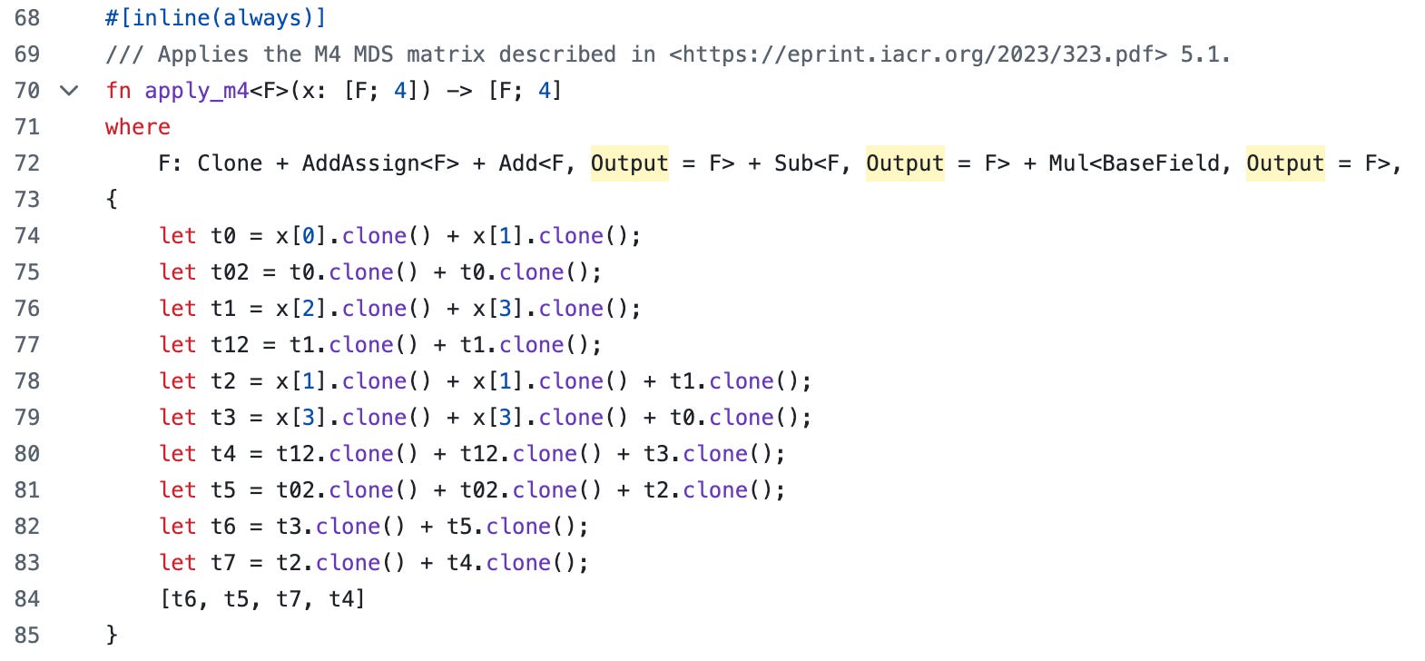
When we write the recursion circuit, we adapt basically the same code and make only a few mechanical edits, as shown below. The mechanical edits include using “QM31Var”—a DSL-powered data structure that is capable of recording operations for DSL—for the variables, and changing the “clone” into passing-by-references.

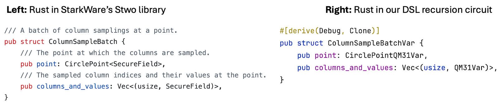
This DSL also allows us to mirror existing data structures and arrays in StarkWare’s Stwo libraries into DSL-powered ones.
For example, in Stwo, we have “ColumnSampleBatch” that is used for arranging the evaluation points and the columns together. We can create a one-to-one mapping in the DSL, called “ColumnSampleBatchVar”, and we can use it in place of “ColumnSampleBatch” when we adapt the code directly from Stwo.
We follow this procedure to implement the entire STARK verifier in DSL. On my 2023 MacBook Pro with the M3 Max chip (which was funded by Starknet airdrop) with 14 cores, it takes about 1 second to 3 seconds to recurse a modest size proof.
To give a concrete number, we ran a benchmark with the following configuration.
The recursion circuit verifies a proof that is also a recursion circuit, with 2^16 rows in the Plonk component, and 2^16 rows in the Poseidon component.
The proof being verified is optimized for prover efficiency and sacrifices verifier efficiency (which is the typical example to use recursion), by using a blow-up factor of 2.
The verification above is repeated 5 times in total.
Here is a breakdown of the number of rows, by each step of the Stwo STARK proof verification, for a single time of the verification (out of five repetitions) .
Fiat-Shamir: 1189 rows in the Plonk component, 840 rows in the Poseidon component.
Composition: 2063 rows in the Plonk component, no Poseidon rows.
Compute FRI answer and decommitment: 176947 rows in the Plonk component, 42720 rows in the Poseidon component.
Folding: 51682 rows in the Plonk component, 120480 rows in the Poseidon component.
It takes 14.27s on my laptop to generate such a proof. On average, it means 2.85s for each proof to be recursively verified.
Note that the recursion time would be different if the proof is for a larger circuit, or if the proof uses a higher blowup factor (which would significantly reduce the verification overhead). Specifically, if we increase the blowup factor from 2 to 4, the amount of work in computing the FRI answer and folding would be halved.
We anticipate that using machines with more cores will further improve the latency—but this probably shouldn’t be the focus of optimization. As we mentioned in the Part I article, the power of recursion is to allow a very large compute task (e.g., verifying a block in Ethereum) to be sliced into many small chunks and be assigned to a large number of instances, where each instance takes care of one or a few chunks.
Then, when the instances complete the proof generation for each chunk, they use recursion to merge proofs together.
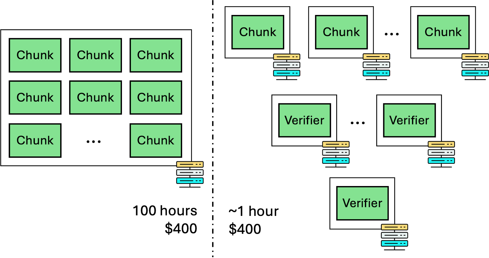
Let us do a concrete calculation. Assuming that the original computation takes about 100 hours to compute. By slicing it into 100 chunks, we can have 100 machines to finish the corresponding chunks in one hour.
Then, we use 20 machines to each merge 5 proofs into a single proof, through the recursion circuit above, which likely takes 15s, and it results in 20 proofs. We then use 4 machines and repeat the same process, which takes another 15s and results in only 4 proofs. We just need to use one final machine to merge the proof, which is approximately another 12s. This only adds an additional overhead of less than 1 minute to the original computation.
As the Part I article says, this fundamentally changes how we scale ZK proofs. Previously, we may try to optimize for single-machine prover efficiency by, for example, using a beefy machine with hundreds of cores. In practice, it has been shown that using many cores doesn’t improve the performance linearly—you may have increased the number of cores from 16 to 192, but the performance improvement is less than 2x.
This is very common in practice and often limits the scalability of single proof generation for ZK. Recursion has been the only approach to break this limitation. Instead of using larger machines, it is both more efficient and more cost-effective to entail a number of smaller machines.
Usage in Bitcoin STARK verifier
The recursive verifier that we have built is also used for Bitcoin STARK verification, which converts a ZK proof that is more prover-efficient to a ZK proof that is more verifier-efficient. By repeating this step multiple times, we can have a proof that is extremely verifier-efficient that is suitable for Bitcoin verification.
Our Bitcoin STARK verifier indeed involves a lot more optimization than what we have covered in this article. Here, we outline them for interested readers, but they all belong to the idea of using recursion to convert a proof from prover-efficient to verifier-efficient.
Switching hash functions. We generate the first Plonk proof using Poseidon hash functions, which is good for recursion, but evaluating the Poseidon hash function on Bitcoin (even with OP_CAT) is not very efficient.
What we do is that, in the last proof, which is the result of layers of layers of recursion, we no longer use Poseidon, but we switches to using SHA-256 as the hash function. Therefore, the Bitcoin STARK verifier, which is implemented in Bitcoin script and uses the Bitcoin execution environment, can simply use the SHA-256 opcode that is available in Bitcoin (subject to the availability of OP_CAT, without which the opcodes would not be as useful).
Although we have been focusing on OP_CAT, and the existing construction relies on OP_CAT, this ability to switch hash functions would also be useful for verifying STARK proofs in BitVM. Currently, in BitVM, we primarily use Blake3 hash functions since implementing it in Bitcoin script turns out to be the easiest. Recursion can also straightforwardly change the hash function from Poseidon to Blake3.
Increasing the blowup factor. We previously mentioned, in this article and in the Part I article, that one can trade-off between the prover efficiency and the verifier efficiency, and that can be done in multiple ways. The easiest way is to increase the blowup factor.
For example, to get the most efficient prover, we use the blowup factor as low as 2. This would require about 80 FRI queries inside the STARK proof verification protocol to achieve a desired level of security. However, we can change this factor while keeping the same security level.
If we increase the blowup factor from 2 to 4, we only need 40 FRI queries.
If we increase it to 8, we need 34 FRI queries.
If we increase it to 16, we need 20 FRI queries
If we increase it to 32, we need 16 FRI queries.
If we increase it to 512, we only need about 9 FRI queries.
Though the verifier efficiency depends on a number of factors, looking at the ballpark number, the fewer the number of FRI queries is, the faster the verifier is. Note that this comes at the cost of a slower prover. For example, when we use a blowup factor of 512, the prover is doing 256x of the work compared with a blowup factor of 2—this is useful only if we are specifically smoothening the proof to be extremely verifier efficient—such as verifying it on Ethereum or Bitcoin as the last layer. In those cases, because on-chain verification could involve an expensive fee, it is financially worthwhile to increase the prover time (only at the last recursion proof) for better performance. In practice, it only takes about hundreds of seconds of computation.
Last-level recursing without Poseidon. Note that the verifier cost depends on a number of factors. The number of columns in the proof system, however, is also one of them.
In the Part I article, we introduced our recursion proof system, which consists of 30 columns for the Plonk component and 96 columns for the Poseidon component. A natural question is whether we can remove the Poseidon component for the last layer (knowing that, as a cost, it would make the prover slower), so that there would be fewer columns.
This is exactly what we do for the Bitcoin STARK verifier where, in the last layer, we use a Plonk component only, but this Plonk component has additional modifications (which can be found here) for processing Poseidon more efficiently without Plonk. Doing so, of course, will increase the number of rows in the Plonk component, and it grows with the number of invocations to the hash function throughout the entire proof verification process—mostly, as we see, from the Merkle trees that are used in decommitment and folding.
The number of the Poseidon operations could become a bottleneck for prover efficiency and in fact, also verifier efficiency. Therefore, we use a new technique to delegate most of the hash operations out to the Bitcoin script, which can be more efficient in evaluating certain hash functions such as SHA-256—of course, not Poseidon. So, we will switch hash functions again, make the “second to last” proof use SHA-256 instead of Poseidon, and then, when the last layer verifies this proof, it delegates the SHA-256 hash operations to Bitcoin. We find that this approach helps us manage the Bitcoin STARK verification cost better.
It is useful to point out that this approach also helps a STARK verifier on Ethereum.
Conclusion
In this article, we continue from the previous article and describe the Poseidon component of our recursive proof system for Stwo. We show why the dedicated Poseidon component can give rise to better performance, and support it with the concrete evaluation.
We are working with StarkWare to integrate the recursive proof techniques built here (for Bitcoin STARK verifier) into StarkWare’s Stwo proof system for settlement to Ethereum and Bitcoin, including BitVM-based Bitcoin bridges.
Find L2IV at l2iterative.com and on Twitter @l2iterative
Author: Weikeng Chen, Research Partner, L2IV
Disclaimer: This content is provided for informational purposes only and should not be relied upon as legal, business, investment, or tax advice. You should consult your own advisors as to those matters. References to any securities or digital assets are for illustrative purposes only and do not constitute an investment recommendation or offer to provide investment advisory services.
Thank you for this series and for releasing your code!
Will you be extending this series to discuss the impact of adding "perfect" zero-knowledge to a recursive STARK? How does the masking step impact the size/cost of the final verifier-efficient proofs?