

In this article we talk about how to implement recursive proof verification in StarkWare’s new zero-knowledge proof system, Stwo. By adding recursive proof verification, Stwo can verify “unlimited” computation and offer developers a flexible choice between prover and verifier efficiency. Our end goal is to make the verifier efficient enough so that Bitcoin, with OP_CAT, can verify it, and therefore bringing STARK verification to Bitcoin. This work is a collaboration with our LP, StarkWare.
Recursive proofs
Before we define recursive proofs, we want to present three challenges in deploying zero-knowledge proofs in production.
The first challenge is memory constraints for large-computation proof generation. When generating a zero-knowledge proof, the larger the computation is, the larger the amount of memory needed, and it can go up to 256GB or 512GB, making it infeasible to fit in most consumer machines or even some cloud instances.
This becomes a serious issue when it comes to zkRollup, which usually runs a zkVM that processes a few blocks. Since each block can have a lot of transactions and each transaction can consume a lot of gas and thereby being computationally heavy, the overall computation adds up very quickly and can go to several TBs. It is infeasible to find machines with such a large memory that can generate a zkVM proof in one shot.

Recursive proofs can help with this by slicing the computation into smaller chunks that can fit into the memory constraints and generating a proof for each part of the computation. In the illustration above, we slice the computation into four chunks and create four individual proofs.
The verifiers can choose to simply verify the four proofs individually and check if the computation has been sliced correctly, but it means that the verifier needs to receive more data and do more work to verify the proofs.
For on-chain proof verification like the case in Ethereum or Bitcoin with OP_CAT, we want to minimize the verifier overhead, so we have another step that creates a proof that consolidates all these four proofs together. Specifically, it proves that:
I know four proofs, each of which is valid, and they are correct slices of a larger computation.
This allows the verifier to only verify one proof, and this proof can be even smaller and easier to be verified than each of the four proofs, if we configure the proof system, here Stwo, properly. What is more, although having recursive verification means that additional proofs need to be generated, they tend to be small proofs that take only a small fraction of the overall proof generation time.
In summary, there are situations when proving a very large computation in one shot and in one proof is infeasible. Slicing the computation into smaller chunks and using recursive proof verification to compose them together solve this challenge.
The second challenge is parallel and distributed proof generation. This is especially useful for zkRollup because even the largest machine available in AWS has only 192 vCPU, and even with a very efficient proof system, it may take a lot of time to generate a proof, and for zkRollup, it would result in a settlement latency.
The latency, however, can be drastically shortened with recursive proof verification. Think that I have some computation that is expected to take one machine 100 hours. I can slice it to 100 chunks, expecting that each chunk takes one hour. Now, if I have 100 machines, I can distribute the proof generation among them as follows:
Let each one of the 100 machines prove one chunk. This takes one hour to finish.
Now, turn off 90 machines, and use only 10 machines. Each machine uses recursive verification to consolidate 10 proofs into one. This takes probably 1 minute.
Turn off 9 machines, and use only one machine. This machine uses recursive verification to consolidate the 10 proofs into one. This takes another minute.
In this way, we generate a proof in one hour plus two minutes, instead of 100 hours, thanks to the ability to distribute the recursive proof generation among multiple machines. The benefit of using cloud servers is that you can scale up and down almost arbitrarily. Math does the magic: the cost of renting a cloud instance to do 100 hours is similar to the cost of renting 100 cloud instances each to do one hour, so you are not even increasing the cost with recursive proofs.

The third challenge is the battle between prover efficiency and verifier efficiency. This has been especially an issue for zkVM and zkEVM because in order to make proof generation efficient, the VM has many application-specific components. For example, zkEVM usually has customized components in the proof system for Keccak256 and elliptic curves. These special components have been indispensable, but they contribute to on-chain verification overhead (which takes $ETH).
One example is CairoVM and its “builtins”, which are special customized components in the proof system that takes care of certain computation. As the very first zkVM in the industry, these designs in CairoVM were inherited in many subsequent zkVM or zkEVM that we see today. In an article “Builtins and Dynamic Layouts”, StarkWare shared some benchmark data on how builtins improve the prover efficiency.
Pedersen is 100x faster to be proven with builtins.
Poseidon is 54x faster to be proven with builtins.
Keccak is 7x faster to be proven with builtins.
EC_OP is 83x faster to be proven with builtins.
However, there is a cost for using builtins, in that the verifier efficiency will decrease. To understand why this is the case for modern proof systems. We need to dive a little deeper on what prover efficiency and verifier efficiency looks like.
In modern proof systems, the computation to be proven is often organized/translated into a table with rows and columns, basically a spreadsheet. Columns are often organized into groups, and they take care of different functionalities. A builtin is usually implemented as a new group of columns.

The proof system defines some relations between the cells in this table. For example,
We can enforce the first column of each row (say column A) to be either 0 or 1.
For every row i, Ai = 0 or 1. I.e., Ai * (Ai - 1) = 0
We can enforce that the third column (say column C) equals the sum of the first column and second column (i.e. addition), say column A and B.
For every row i, Ci = Ai + Bi
We can enforce that the fourth column (say column D) equals to the third column (say column C) in the previous row.
For every row i, Di = C{i-1}
These are just simple relations. When we deal with hash functions like Keccak256 or SHA256, chances are that it would consist of hundreds of columns and a long list of such arithmetic relations.
How does the table relate to the prover efficiency and verifier efficiency? Say that the table has X rows and Y columns.
Prover’s work in generating the proof is largely related to the number of cells in the table, i.e., X * Y, number of rows times number of columns.
Verifier’s work in verifying the proof is linear to the number of columns, but only logarithm to the number of rows, i.e., Y * log(X). Specifically, the verifier’s work relates to the complexity of all the arithmetic relations that need to be checked.
Builtins are effective for prover efficiency because although they increase the number of columns, the net total of the number of cells are significantly reduced. This, however, usually leads to increased verifier overhead, simply because there are more columns and the relations between the columns get more complex.
Recursive proof verification comes to rescue. The idea is that, for sufficiently large computation, it is always “better” if we use a hybrid of two proof systems:
The first proof system is optimized for prover efficiency, with a modest verifier efficiency. The proof from the first proof system is not going to be verified on-chain.
The second proof system is optimized for verifier efficiency and is specifically designed for verifying proofs from the first proof system. The proof from this second proof system will be verified on-chain.

Note that other than the need to design two proof systems to fulfill this purpose, there is really no downside for playing with two proof systems. One just gets improved prover efficiency and verifier efficiency altogether. This idea was originally from Madars Virza from MIT called zk-SHARKs in 2019 and has since evolved to be a standard practice.
Design recursive proofs in Stwo
In recursive proofs, the core task is to build a proof system that is used to verify a Stwo proof (i.e., run the computation of a Stwo verifier).
Designing this dedicated proof system is not trivial because a naive implementation could easily lead to a recursive proof that is larger than the original proof, making the final proof “harder to verify”. This is especially the case for hash-based proof systems because hash functions tend to be very expensive to verify in ZK proofs.
There is flexibility in picking hash functions. Stwo can work with many hash functions: Blake2s, Blake3, Poseidon2, and SHA-256. Among these hash functions, Poseidon2 is easiest to be verified, but running Poseidon2 in a naive proof system (that does not have Poseidon2 builtin) can easily be inefficient.
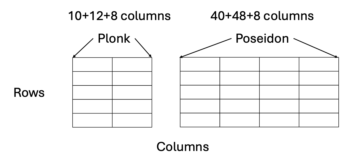
So, we build a proof system over Stwo that is dedicated to verifying Stwo proofs. It consists of two components: (1) Plonk and (2) Poseidon. Most of the logic of a Stwo verifier is implemented in Plonk, but whenever the verifier needs to compute a Poseidon2 hash, it delegates it to the Poseidon component. The two components are connected to each other through the LogUp checksum from Ulrich Haböck.
We believe that this is a fairly tidy and well-crated design, and we will show later that it delivers favorable performance. In this article series, we aim to provide you with the details of these components. Here we go!
The Plonk component has 10 + 12 + 8 columns:
The first 10 columns are called “preprocessed” columns. They are descriptions of the Stwo verifier and do not depend on the proofs, so the prover can compute them once and doesn’t have to compute again. They are listed as follows: “a_wire”, “b_wire”, “c_wire”, “op”, “mult_a”, “mult_b”, “mult_c”, “poseidon_wire”, “mult_poseidon”, “enforce_c_m31”. We will explain their meanings soon.
The next 12 columns are called “trace” columns. Every 4 columns represent a degree-4 extension of the M31 field element, where M31 means a number modulo the Mersenne prime 2^31 - 1. This is the basic unit of computation in a Stwo verifier. So, the 12 columns represent three such numbers, called “a_val”, “b_val”, “c_val”. We will soon discuss what they are, but the Stwo verifier computation is defined over this degree-4 extension.
The last 8 columns are for LogUp checksum that connects different rows in the Plonk components together as well as connects the Plonk component to the Poseidon component.
The Poseidon component has 40 + 48 + 8 columns:
The first 40 columns are also “preprocessed” columns. They are independent from the input and output of the hash functions, but rather, it provides some descriptions.
It starts with four columns “is_first_round”, “is_last_round”, “is_full_round”, “round_id” that describe whether this row corresponds to the first round, the last round, and/or a full round in the Poseidon2 hash function as well as the round index.
It is followed by 32 columns for round constants of the Poseidon2 hash function.
Finally there are four columns “external_idx_1”, “external_idx_2”, “is_external_idx_1_nonzero”, “is_external_idx_2_nonzero” that indicate which row in the Plonk component should correspond to this row—which connects the two components together.
The next 48 columns are “trace” columns. It consists of three Poseidon2 states (each state has 16 elements), one as the input state, one as the intermediate state, and one as the output state.
The last 8 columns, similarly, are for the LogUp checksum.
In this article, we will focus on the Plonk component and talk about how it works, as well as why we designed it in this way. In the Part II article, we will discuss more on the Poseidon component. And in the Part III article, we will devote ourselves to how to build a Bitcoin-verifier-friendly proof system, which involves some niche details only of interest to Bitcoin.
Arithmetic relations between A, B, C
We start with the most intuitive part of the Plonk component. This involves a preprocessed column “op” and 12 trace columns forming degree-4 extensions “a_val”, “b_val”, and “c_val”.

It can be then used to define addition and multiplication relationships between these values.
When op = 1, we have C = A + B
When op = 0, we have C = A * B
When B = 0, we have C = op * A, which can be seen as multiplying A with a proof-independent constant op
With additions and multiplications, one can perform the rest of the arithmetic operations.
Subtractions like A - B can be done by first negating the subtrahend B by multiplying it with -1 and then adding A and (-B) together.
Divisions in the prime field A / B are often defined as A * (B^-1) where B^-1 is the multiplicative inverse of B such as B * (B^-1) = 1. This is done by presenting the modular inverse, using B * (B^-1) = 1 to check that it is the correct modular inverse, and then multiplying it with A.
However, there are two issues with this simple relation.
We start with the easier one. Note that A, B, C are all on the degree-4 extension of the M31 field, called QM31. An element in QM31 can be written, similar to complex numbers, as:

where i and j are units. A can also be viewed as a vector [a0, a1, a2, a3].
Although we can perform all kinds of operations over QM31, there is almost no way to enforce that an QM31 element is also a M31 element (i.e., a1 = a2 = a3 = 0). This is, however, necessary in the Stwo verifier, as some elements are supposed to be M31 rather than QM31.
To do this, we have another column, “enforce_m31”, which enforces C to be an M31, meaning that the second, third, fourth columns that represent “c_val” should be zero.
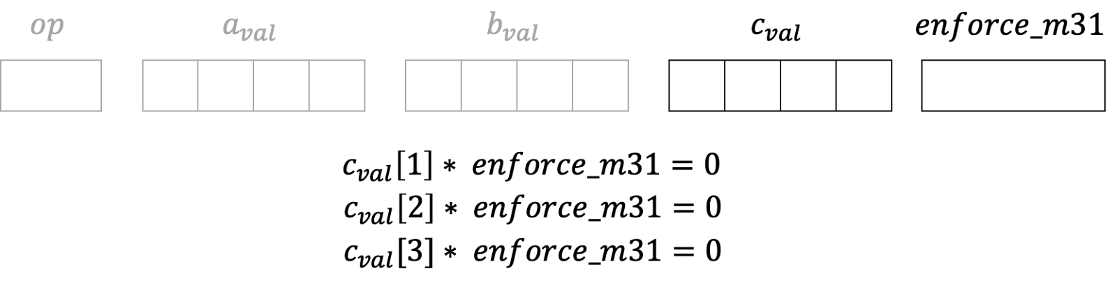
Although “enforce_m31” only enforces C, we will soon show how it can be used to enforce A and B to be M31 elements in an indirect way. This is exactly the other issue.
As one can see, although we can do a single addition or a single multiplication in one row, to be able to fit in more complicated computation, even subtraction and division, we will need to use more than one row, where the result C in a row could become input A in the other row.
But at this moment, we do not have a way to enforce that C here becomes A in another row. This is necessary for subtractions because subtrahend multiplied by -1 would need to appear in another row to compute the difference.
This is where “wire IDs” come into play, where for each value, we assign an ID. Values from the same ID, which could be in different rows, must stay the same. In this way, different rows can be connected together.
So, as the figure below shows, in each row, there are now three preprocessed columns “a_wire”, “b_wire”, “c_wire”. They are the corresponding wire IDs of A, B, and C.

Values with the same IDs, which could be in the same row or in different rows, must have the same value, so one row can now “continue” the computation unfinished by another row. The guarantee that values with the same IDs must be the same is enforced by the LogUp technique as follows.
Use LogUp to connect values across rows
LogUp is a technique by Ulrich Haböck, proposed in 2022, that can be used to connect values (and their IDs) across different rows in the table.
The idea is that, if all the values and IDs are consistent, we can derive “mult_a”, “mult_b”, “mult_c” for each row that satisfy the following equations.

In this equation, H is a random and unpredictable hash function that is selected by the verifier. Basically, this hash function would output the same number if the two inputs—wire ID and the value—are the same, but this number would be random and cannot be predicted by the prover. That is to say, if two inputs have the same wire ID but different values, their outputs from this hash function will be different, and the prover cannot predict the difference between the outputs.
“mult_a”, “mult_b”, “mult_c” can be set purely based on “a_wire”, “b_wire”, and “c_wire”. For example, if a specific wire ID has been used for 16 times in the entire table (which could be in positions A, B, or C), we can set the first “mult_X” value for this wire ID to be “-15”, and all the remaining “mult_X” for this wire ID be “1”. In this way, across the table, all the fractions with respect to this wire ID will add up to zero.
If all the wire IDs are being configured correctly in this way, then the total sum as above will also be zero.
Now, if there is any input that the wire ID and value have inconsistency, the LogUp paper proves that the sum will not be zero, with an overwhelming probability, thanks to the unpredictability of the hash function. This hash function can be concretely constructed using two random variables, “α” and “z”, both of which are chosen by the verifier after the prover has committed all the trace columns.

To compute the checksum of the entire table, there are 8 more columns used to aggregate the sum, and every 4 columns represent the intermediate aggregated result. We denote them as “sum_1” and “sum_2”.

As the figure shows, “sum_1” is simply the sum of the fractions for A and B, and “sum_2” adds the fraction for C and the previous row’s “sum_2” into “sum_1”. And the LogUp technique cleverly leverages a trick that in Circle STARK, the previous row of the first row of the table is “defined” as the last row of the table, so the first row will also add “sum_2” of the last row of the table. It can be shown that if the “sum_2” relation can be satisfied even in this circular manner, then all fractions for A, B, C in all rows add up to zero. Below is an example where the first row has sum_2[0] and the last row has sum_2[7]. The computation of sum_2[0] will involve sum_2[7], but sum_2[7] also depends on sum_2[0]. This can only happen when the total sum is zero.

Note that there are still “poseidon_wire” and “mult_poseidon” which will be involved in “sum_2” as well that we omit for now. They are used to enforce consistency on values shared between the Plonk component and the Poseidon component, and we will discuss that in Part II.
Next steps
In this article, we presented the design details of the Plonk component, the design of which can be summarized as two parts. One part takes care of the basic arithmetic operations (additions and multiplications) for three values A, B, and C within a row, and another part takes care of enforcing consistency between values under the same IDs across rows using the LogUp technique.
In the next article, we will dive into the design of the Poseidon component as well as how it interacts with the Plonk component. After presenting the two components, we will show how the recursive verifier can be implemented within these two components.
Find L2IV at l2iterative.com and on Twitter @l2iterative
Author: Weikeng Chen, Research Partner, L2IV
Disclaimer: This content is provided for informational purposes only and should not be relied upon as legal, business, investment, or tax advice. You should consult your own advisors as to those matters. References to any securities or digital assets are for illustrative purposes only and do not constitute an investment recommendation or offer to provide investment advisory services.